Methodology
The methodology differs in the multiphysics coupling
i). Fully coupled model
- assuming lithostatic total pressure gradient => decoupling of the fluid flow from shear deformation
- prediction of stresses and pressure distribution in the porous matrix (geomechanics)
Benifit 1: Total pressure does not follow a lithostatic gradient?
Benifit 2: The shear deformation of the porous matrix is resolved?
a). Direct coupling (Industry-related simulator)
- fluid pressure is transferred to the geomechanical module, but the geomechanics do not impact the fluid pressure
b). Iterative coupling
- iterative coupling of the fluid-flow solver to a geomechanical solver
c). Single solver
- fully coupling of the fluid flow and the Stokes matrix flow within a single solver
ii). Decompaction weakening model decompaction weakening while coupling Darcian and Stokes flows in 3-D
Decompaction weakening Räss et al. (2019)
Motivation
study of various phenomena of porous fluids (fingering, veining, channeling and focussing)
structure: subseabed pipes (eg. on the Nigerian continental shelf and in the Norwegian North Sea)
may act as preferential fluid pathways. Understanding how these pipes are formed and evolved can help us to accurately constrain subsurface fluid flow
[] What is the delocalization of the patterns of the flow?
Experiences: flow patterns are localized, induced by fractures
Theory: using classical Darcian model, diffusive behavior is expected => leads to never-ending spreading and delocalization
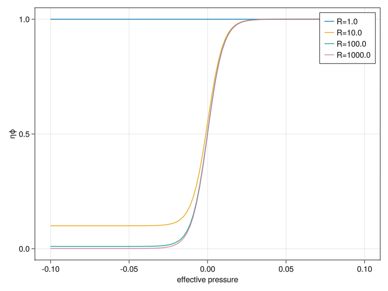
What is the decompaction weakening?
corresponds to high $\eta_d$ value
The degree of the decompaction weakening can be quantitatively determined by the quotient of the compaction bulk viscosity $\eta_c$ and its decompaction counterpart $\eta_d$.
\[R = \frac{\eta_c}{\eta_d}\]
Decompaction is significant $R >> 1$ => flow channeling
when $R=1$ we have blob-like porosity waves
The effective pressure $P_e$ can be used to monitor the compaction within a certain region.
Region in compaction $P_e > 0$
Region in decompaction $P_e < 0$
Mathematical model
Bulk viscosity
\[\eta_{\phi} = \eta_c \frac{\phi_0}{\phi} [1 + \frac{1}{2} (\frac{1}{R} - 1)(1 + \tanh [-\frac{p_e}{\lambda_p}])]\]
Numerical experiment
Media: fluid-saturated
Objective: observation of the flow patterns
- localized, delocalized?
formation?
propagation?
Numerical methods
The PT-method used in Räss et al. added the non-linear residual terms $f_v, f_{p^{[t]}}, f_{p^{[f]}}$ to 3 of the governing equations and aims to obtain the solution by minimizing the residuals iteratively within a pseudo-time loop
Results
Decompaction weaknening
3x-higher fluid-flow rate than the pure Darcy model